Welcome to another blog where we look at Machine Learning in Production. This is an ongoing series looking at deployment options for Machine Learning models.
We are making our way closer to having model which we can put in to production with Docker and Kubernetes. In this blog we are going to do the following:
-
Learn a little about regression modelling
-
Pull a dataset from GitHub
-
Clean the dataset
-
Create a machine learning model to predict the price of a house
In this blog we are going to look at building a basic model in Python. Feel free to build this model or another in any language of your choosing. I am often asked which language they should learn when you're getting started - most ask Python or R, the simple answer is that both are good, but in different ways. I recommend learning both and using the best tool for the job you have and what works for the skills that the rest of the team have.
The problem - Predicting the value of houses.
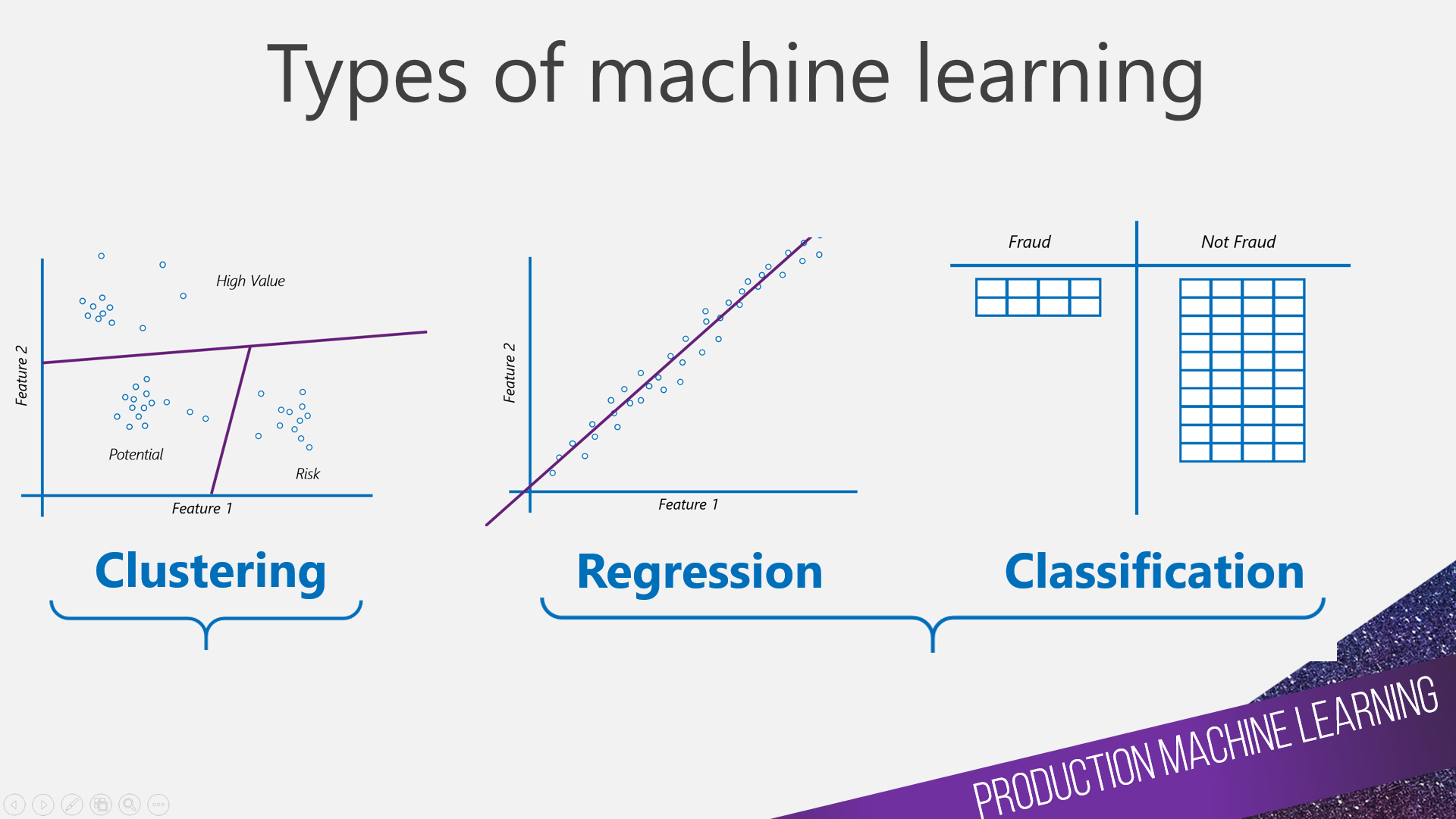
There a many types and categorisations of machine learning. The following image shows you examples of three common types used in shallow machine learning.
-
Clustering - Unsupervised data mining (we do not have a label to predict), typically looking to group the data you have in to clusters. K-means is an example of a clustering algorithm.
-
Regression - Supervised machine learning (we have a label). We are looking to predict something which is numerical. Linear regression is an example of a regression algorithm.
-
Classification - Supervised machine learning (we have a label). We are looking to predict something with is not numerical, it is categorical. Decision Tree is an example of a binary classification algorithm.
For this blog an the model we are looking to create, we will focus on regression. Below is an example of what linear regression looks like. The moustached gentleman is a typical customer. They have some data, and a problem, but they are not too sure where to go next. The customer is explaining "I am trying to predict how much someone will spend next time they come to my store". To distil this down further, they are trying to predict spend - spend being numerical - the amount spent. We are going to look to plot a straight line between a number of features (attributes), we will then use the intersection of those points is what we will predict.

Continuing with our problem.
You're a data scientist, working for a large Estate Agent/Realtor. You have a dataset which contains the prices each house was sold for and 80 features which may or may not contribute to the value of a property. We are going to build a model which will predict the price of a house based on a handful of key predictors. This is all based on the Kaggle house price dataset.
We will build our model in Python using Sci-kit Learn, however you could build the same model in R if you wanted.
You can just grab the code if you want to or you can step through building the model step-by-step. Now the purpose of this blog is not to teach you how to master machine learning, it is designed to take a simple problem and show you how to go about getting that model in to production. We are focusing on a shallow machine learning model for this example, but later we will do the same as we are about to, but with Deep Learning. I will explain what is happening and give you justification for the process, but I am 100% sure you could improve on the models accuracy - and I think that you should!
In this blog we are just looking at the Data and the Python element of the model creation. In the next blog we will discuss serialisation and API management. You can build this model in any ide you wish. I will be using VS Code and the Anaconda distribution. In screenshots you will also notice that I use multiple environments, which I manage with Conda. Conda is a package management tool for Python. Managing dependencies in any language is hard, so having a tool which can ensure that the versions of a package running on your machine, are the same as those on the production machines - what happens if they are not? Simple answer, deployments fail.
Installing packages
If you have never looked at machine learning before, or you're using a new machine you will most likely not have all the required packages to be able to run this script. Well that is a simple fix. If you're using Anaconda, then open an Anaconda Prompt window, if you're using linux or a mac open a terminal. Enter the following:
For pip it is the following:
Pip install pandas For Condas it is the following.
Conda install pandas Some times you will need to tell the terminal window that you're using Python and you would do that as follows:
Python -m pip install pandas. I have mentioned about the importance of package management what we have just done is not great. By asking to install pandas we are saying go and install the latest good version of Pandas. When you run a pip install the version you pull is the latest version available at the time of issuing the command (0.24.2 - latest version today). Now the problem of working in this way is that when you install Pandas today when you come to deploy the model to a server or remote service then the versions may be different, and some of the features you require are not available or function in a different way. We can resolve this by locking each package down to a particular version number.
Python -m pip install pandas==0.24.2Python -m pip install numpy==1.16.3Python -m pip install scikit-learn==0.21.0Create a new python script and add the following:
# Import the packages
import pandas as pd
import numpy as np
import math
from sklearn import metrics
from sklearn import linear_model
from sklearn.model_selection import train_test_split
Importing data, cleaning data and label encoding
Now we have the packages we need, next we need to grab some data and build the machine learning model. Machine learning is as much an art as it is a science. I say this because getting a set of data from its raw format to the point where it generalises and allows for machine learning is complicated. There are so many techniques and tricks you can apply. Knowing all of them is a science, knowing how to apply them in new and interesting ways, to me feels more like an art. I will show you a few little ways we can improve performance on our model, this is to make the model a little better and again, it is not designed to teach you machine learning.
Add the following code to download the data from my github and then create a Pandas DataFrame. A DataFrame is a lot like a table in a relational database. If you're familiar with this data structure then DataFrames will look very familiar. This is why we are using Pandas. Pandas has a huge amount of amazing functions, the best being the implementation of DataFrames.
Add the following code below the package installation.
# Download the data
train_url = "https://raw.githubusercontent.com/SQLShark/pluralsight-data-science-version-control/master/Notebooks/data/houseprices/train.csv"
train_df = pd.read_csv(train_url, error_bad_lines=False)
The data we are working with has 81 features. To simplify the training process, we are going to limit these down to a handful of the key predictors. We can investigate the key predictors with a correlation plot. For this I have used Seaborn. Seaborn is an impressive data visualisation package. What you can see in the image below is how correlated each feature is to the label (SalePrice). The lighter the cell the more correlated it is.

We are going to limit the dataset down to the following features:
-
YearBuilt
-
GrLivArea
-
GarageCars
-
SaleCondition
-
BldgType
-
OverallQual
SaleCondition and BldgType are both categorical features - they have string(text) values and not integers(numbers). Machine learning algorithms do not work with strings, they need integer representations of the string values. We will provide this with a process known as label encoding. You can use a function in SKLearn for this. Or we can do it manually. Manually is a good way to show off a different approach, so we will do that. In production where you have changing value this might not be possible.
Add the following code below the previous section.
# Label encoding
SaleConditionMapping = {"Normal":1, "Abnorml":2, "Partial": 3, "AdjLand": 4, "Alloca": 5, "Family": 6}
BldgTypeMapping = {"1Fam":1, "2fmCon":2, "TwnhsE": 3, "TwnhsE": 4, "Twnhs": 5}
Each time we see the string value "Normal" for SaleCondition, we will replace it with a 1. To apply this we will need to map it to a new column in our DataFrame. In the next section we will do that and also clean our data a little and impute some missing values.
Add some more code:
combined = [train_df]
for dataset in combined:
dataset['SaleConditionMapping'] = dataset['SaleCondition'].map(SaleConditionMapping)
dataset['BldgTypeMapping'] = dataset['BldgType'].map(BldgTypeMapping)
dataset['BldgTypeMapping'] = dataset['BldgTypeMapping'].fillna(1)
dataset['SaleConditionMapping'] = dataset['SaleConditionMapping'].fillna(1)
dataset['GarageCars'] = dataset['GarageCars'].fillna(dataset['GarageCars'].mean())
dataset['OverallQual'] = dataset['OverallQual'].fillna(dataset['OverallQual'].mean())
Here we are mapping the integer values back to our DataFrame. We are also imputing some missing values. Here we are replacing SaleCondition and BldgType with the first and most common value. We are then imputing the mean for GarageCars and OverallQual and updating the values. This is all in an attempt to provide our model with the best ability to predict something which is generalised to our problem.
Selecting an Algorithm and training a model
Now we are ready to build a model. This is actually the simple part. The hard work has been completed. First we need to split our data in to a train and a test set. This is for the purpose of evaluation. We are looking at Regression models, so we will be using a loss function called Root-Mean-Squared-Error to evaluate how well our model is doing. We will hold back a percentage of our data to ensure that we can calculate the RMSE.
Add the train-test split logic:
The gif below shows what we are looking to do here.
Next we need to select an appropriate algorithm and train our model. I will be using a BayesianRidge regression model. I select the model and then train the model by calling fit and providing the features and the label for my data. I then pass in the test data I held back and get the predictions. I will then used this to calculate the loss function.
Add the machine learning element:
# Machine learning
br = linear_model.BayesianRidge()
br.fit(X_train, y_train)
y_pred = br.predict(X_test)
Loss function checking
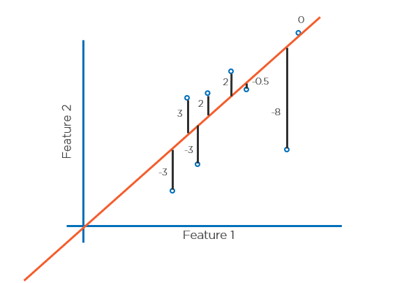
To evaluate the success of our model we need to calculate the loss of our model, this then indicates how accurate our model is. We will be using root mean squared error, which starts with the mean squared error. Refer to the image below and you will see a straight line applied to a set of data. To calculate the MSE we will need to calculate the distance from the prediction and the actual. Then we square each of the numbers and add them up and take the average. The smaller this number the better - but you need to know your data.
Example:
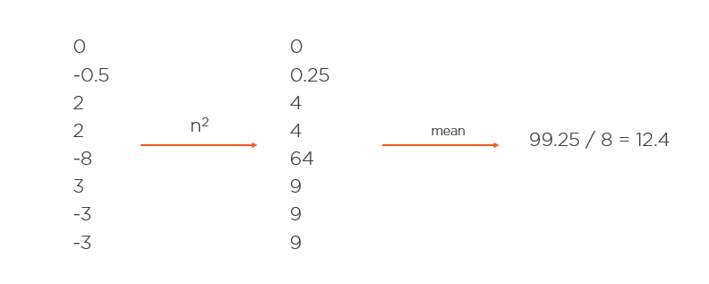
This is a good indication, but because the number has been squared, it is hard to know how well the model is doing. To make this number more understandable we can take the root of it. Doing this will bring it back in to terms we can understand in the context of the model we have created.

Add this all together we have a MSE of 3.5 for the images we have been looking at. Looking at the average loss in the image above, this feels representative of our data.
Add the following code to see how well your model has performed:
# Error checking
error = metrics.mean_squared_error(y_test, y_pred)
print("MSE:",error)
print("RMSE:", math.sqrt(error))
When I run this model I get a RMSE of 40100, which is to say that my model on average is 40K out in its prediction. That may seem like a lot, however the mean value for SalePrice is $180,000, therefore $40,000 is 22%. Our model is roughly 78% accurate. This might be acceptable, but we could improve on this with multiple iterations.
For now, we will leave this here. In the next blog we will take our model and serialise it, then add a REST API so we can call it.
Completed code:
# Import the packages
import pandas as pd
import numpy as np
import math
from sklearn import metrics
from sklearn import linear_model
from sklearn.model_selection import train_test_split
# Download the data
train_url = "https://raw.githubusercontent.com/SQLShark/pluralsight-data-science-version-control/master/Notebooks/data/houseprices/train.csv"
train_df = pd.read_csv(train_url, error_bad_lines=False)
# Label encoding
SaleConditionMapping = {"Normal":1, "Abnorml":2, "Partial": 3, "AdjLand": 4, "Alloca": 5, "Family": 6}
BldgTypeMapping = {"1Fam":1, "2fmCon":2, "TwnhsE": 3, "TwnhsE": 4, "Twnhs": 5}
# Clean the data and apply label encoding
combined = [train_df]
for dataset in combined:
dataset['SaleConditionMapping'] = dataset['SaleCondition'].map(SaleConditionMapping)
dataset['BldgTypeMapping'] = dataset['BldgType'].map(BldgTypeMapping)
dataset['BldgTypeMapping'] = dataset['BldgTypeMapping'].fillna(0)
dataset['GarageCars'] = dataset['GarageCars'].fillna(dataset['GarageCars'].mean())
dataset['OverallQual'] = dataset['OverallQual'].fillna(dataset['OverallQual'].mean())
# Test train split
X = train_df[['YearBuilt', 'GrLivArea','GarageCars','SaleConditionMapping','BldgTypeMapping','OverallQual']]
y = train_df[['SalePrice']]
X_train, X_test, y_train, y_test = train_test_split(X, y, test_size=0.3, random_state=42)
# Machine learning
br = linear_model.BayesianRidge()
br.fit(X_train, y_train)
y_pred = br.predict(X_test)
# Error checking
error = metrics.mean_squared_error(y_test, y_pred)
print("MSE:",error)
print("RMSE:", math.sqrt(error))