


Understanding how Prophet does what it does.
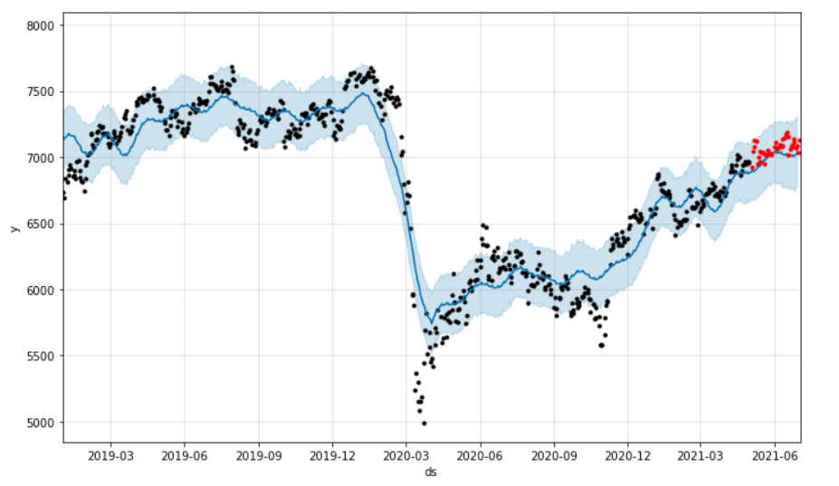
Prophet-generated FTSE100 fitting and forecast.
This post is a follow-on from the previous article, where we used a simplistic Prophet model to forecast the FTSE100 index. In this post we will take a look at some of the inner workings of the Prophet model to understand exactly how the forecasts are made.
Prophet’s components plot
Using the FTSE100 example from before, we can call model.plot_components( forecast_df ) to produce the below graphs.

Prophet-generated component plots.
These plots give us a little insight into how the model is formed. The trend plot (top) exhibits a linear, piecewise function, with approximately appropriate values for our dataset throughout the years. This looks to be a baseline for predictions.
The weekly plot (middle) demonstrates some interesting behaviour - weekdays have a small negative impact on the predictions (approximately -50), and we see large spikes for the weekends. This appears peculiar, as we have no weekend data in our dataset, but it is a product of fitting a 7-day periodic function to only 5 days of data. Thankfully, this won’t be an issue as we have no need to forecast weekends.
The yearly plot (bottom) shows a much more volatile impact on predictions (-200 to +180) with frequent changepoints throughout. This points to a more sensitive and complex relationship between the time of year and the FTSE100 index than the day of the week.
How is Prophet formulated?

LaTex representation of the Prophet forecasting function.
Prophet accepts a dataframe with a minimum of two columns, “ds” our timestamp, and “y” our target variable. This makes some sense as the above formula displays only functions dependent on t (time).
y(t) is our function and simply describes the prediction.
g(t) is our trend function, this can be either a piecewise linear or piecewise logistic trend. (You can opt for growth = ‘flat’ to remove any trend-fitting here, although this will produce large uncertainties in any non-flat datasets.)
s(t) is our seasonal function, this is a Fourier series approximation to the intra-daily, weekly or yearly seasonal components. These are automatically set upon detection of intra-daily/weekly/yearly data.
h(t) is our holiday/events function. Prophet accepts a dataframe of dates, and upper/lower windows where the time-series is possibly affected by these events. These were omitted in the base model.
ε is our error terms, these are assumed to be normally distributed.
The trend function
The trend function typically takes one of two forms, piecewise linear or piecewise logistic growth trends. In the FTSE100 forecast, a linear piecewise approximation was used (and rightly so, as modelling most financial instruments as logistic growth is a dangerous practice…).
Linear growth
Linear growth is typically modelled as some variation of:

Where f(t) is our approximation, k is our growth rate, t is time and m is some offset value, to accommodate varying windows of our dependent variable, t.
The example below has a growth rate (k) equal to 1, and an offset (m) equal to 2.

Simplistic linear growth plot.
Prophet extends this model, and uses compact notation to describe the complexities in extending it towards a piecewise linear growth model:
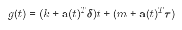
Prophet’s linear growth model.
The formula has gotten a lot more complex, but a lot of the complexity arises from formulating an equation describing multiple trend approximations.
Firstly we recognise the similarity in the equations, the above is just an extension of the typical linear growth equation, so we will only discuss the discrepancies.
The vector a(t) represents binary outputs that signify which growth rate adjustments are valid for that point in time. It is an “on/off” switch for our growth rate (and offset parameter) adjustments. It is transposed to allow for valid vector multiplication with the aforementioned vectors.
The vector δ represents our vector of growth rate adjustments, if we have 5 different linear growth rates, this will simply contain the 5 different values for our growth rate adjustments (k gets adjusted by the value in δ). Multiplying by our (transposed) a(t) vector simply yields the correct growth rate adjustment for that point in time.
The vector τ represents our adjustments to the offset parameter (m). In the same way as our δ vector, when multiplied by our (transposed) a(t) vector yields the correct growth rate adjustment, this yields the correct offset parameter adjustment to connect the endpoints of the linear “pieces” that form our piecewise function.
To put it simply: the formula above just describes how to piece together multiple straight lines to form our (linear) piecewise trend function.
Logistic growth
Logistic growth is typically modelled as some variation of:

Typical logistic growth equation.
Where f(t) is our approximation, C is the carrying capacity, or the ceiling to our population, k is our growth rate, t is time and m is some offset value, to accommodate varying windows of our dependent variable, t.
This model approaches and plateaus at C as our exponential term (e) approaches 0. The example below illustrates a carrying capacity (C) of 10, a growth rate (k) of 1 and an offset (m) of 0.

Simplistic logistic growth plot.
Prophet extends this model further, resulting in the below equation:
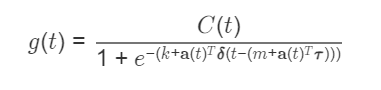
Prophet’s logistic growth model.
This compact notation (again) encodes the entirety of the logistic growth model for Prophet. The complexity is once more down to the representation of multiple curves.
Our constant carrying capacity, C, becomes C(t) signifying that it is dependant upon time, rather than a constant. The other amendments to the formula are exactly as described in the linear growth section.
To put it simply: the formula above just describes how to piece together multiple logistic curves to form our (logistic) piecewise trend function.
Automatic trend changepoint selection
Prophet automatically selects changepoints for the growth rate. This is achieved by generating a uniform set of “A” changepoints (default of 25) inferred from the first “B” percent (default of 80) of our dataset. A sparse (Laplace) prior is applied as below, where the parameter τ allows us to directly control the frequency of non-zeros. This in turn, controls the number of the potential trend changepoints that end up being used.
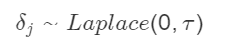
Laplace prior.
If we return to our original model, we can access the 25 potential trend changepoints inferred from the first 80% of our dataset.

Prophet’s potential trend changepoints.
We can then compare this plot to the selected trend changepoints.
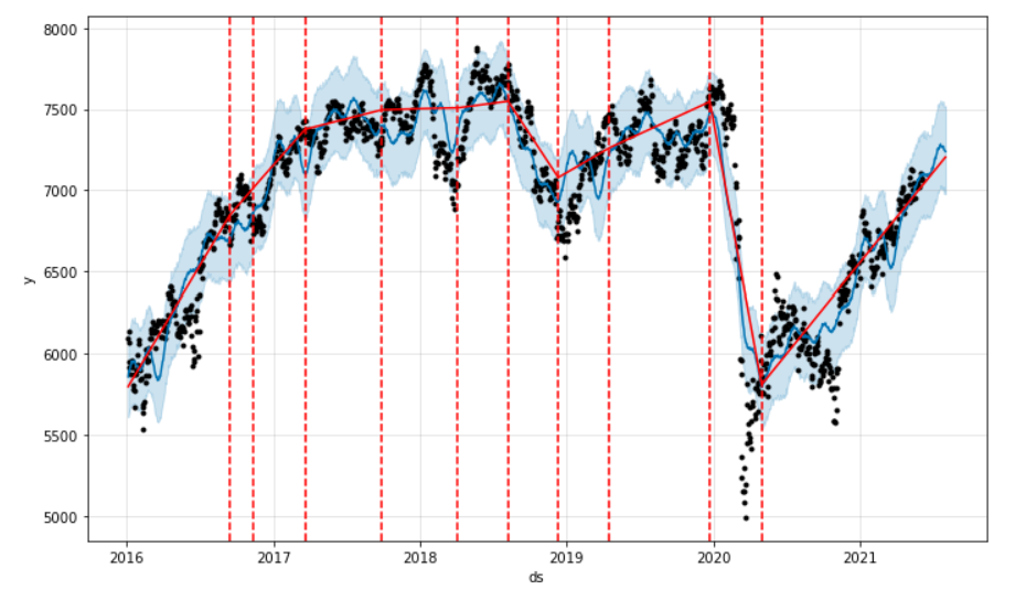
Prophet’s actual trend changepoints.
We can observe the reduction from 25 potential changepoints to our 10 finalised ones. It’s important to note here, that as τ approaches 0, the model will select no trend changepoints, this means the fit will be done with the original growth rate (k), and will resemble a standard linear/logistic growth model, rather than the piecewise model we’ve discussed here.
The seasonal function
The seasonal function is composed of Fourier series approximations to our intra-daily, weekly and yearly trends. In the FTSE100 example, as we have no intra-daily data, only weekly and yearly trends are approximated in this way. Fourier series approximate a function (or signal) by taking a sum of sine and cosine waves, as below.
![Fourier series definition on the interval [0, L].](https://images.squarespace-cdn.com/content/v1/5bce4071ab1a620db382773e/1627652871430-9CRGRNNGE8KMRLPUOL1U/fourier_def.png)
Fourier series definition on the interval [0, L].
If the notation is off-putting, hopefully a simple example of approximating a “sawtooth signal” helps demystify this process. The red line is the signal we’re attempting to approximate, and the blue line is our Fourier series approximation. We increase our number of terms from 2 to 10 to 50.

Fourier series approximation.
As the graphs above demonstrate, as the number of terms increases (or approach infinity) the approximation gets closer to the original signal. This increase in the number of terms means more “high-frequency” waves are included in the approximation, resulting in the large number of oscillations in our 50-term plot.
Prophet’s default behaviour is to fit weekly seasonality with 3 terms, and yearly seasonality with 10 terms. These few terms enforce fitting to low-frequency seasonal trends, making the model less sensitive to large, sharp, seasonal fluctuations and potential overfitting.
Once the seasonal components are approximated using Fourier series, a smoothing prior (below) is applied to generate the seasonal component of the model, s(t).

Smoothing prior.
The holiday function
Prophet allows for user-defined input of custom dates to signify relevant events to the dataset. This is useful where the analyst has domain-specific knowledge that can help aid in forecasting. Prophet’s library also contains a list of country-specific (and agnostic) holidays, along with potential ranges of their effects on the model.
While we didn’t use holidays in our initial model, we can import the (inbuilt) UK holidays and display them.

Prophet’s country_name = ‘UK’ holidays.
With specified holidays, a date range is constructed around them, allowing each holiday to affect a range of dates either side. A parameter (for the change in forecast) is assigned to the days in the specified range. A smoothing prior (below) is then applied.

Once a model has been fitted to the training set, when we display our components plot, we now also have a plot for holidays. These impact the model exactly like the trend function and the seasonal function, where we take the sum (for additive models, product for multiplicative models) of each of our functions, and you have your model!

Prophet’s holiday component plot.
Summary
While Facebook Prophet offers a quick, intuitive way to forecast time-series data, it can be helpful to understand some of the inner workings of your models. Hopefully this article has demystified a little of Prophet’s magic. The next article will discuss hyperparameter selection, using some of the understanding of the model we have gained here.