


If you keep up with the latest developments in the data space, you will probably know that Microsoft Fabric has now reached general availability. While it clearly still needs some more features it seems like Microsoft are fully behind Fabric and it will be an important product for them going forward.
At Advancing Analytics we have been lucky enough to have access to Fabric during its preview and have even started to develop our own Fabric accelerator. Feel free to contact us if you want to know more!
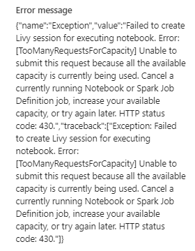
One of the most difficult things during this process for us was understanding how concurrency works and how we can run multiple notebooks at once without getting errors. It seemed like whenever we tried to run two notebooks at the same time, we would always get concurrency errors like this one.
The reason lies in the documentation in the snippet below.

Currently this means if you exceed your capacity for interactive jobs, you will just receive an error message and your activity will fail. Currently this seems to be a real weakness with Fabric and it’s something I hope Microsoft will be fixing soon.
What is capacity?
If you are currently using Microsoft Fabric you will have some sort of capacity associated with your account. This will have a large impact on what you can run concurrently. If you are on a Fabric Trial, you will have access to a trial capacity and if you are paying you will be on a certain capacity tier based on how much you pay. The following diagram shows information about each level of capacity and the Trial. The Trial resembles F64 capacity but is apparently different in some important ways (More on that later).

If you have searched for information about Fabric concurrency you have probably seen the above diagram from Microsoft’s documentation. I was immediately confused by it and made some assumptions that turned out to be wrong. This diagram is key to working out available Notebook concurrency and unlike the diagram itself the method is thankfully simple.
What is an Interactive job compared to Batch?
The first important concept from the diagram which can be misleading is the concept of Interactive and Batch. The following diagram from the Docs explains the difference.

Looking at the above table we can see that notebooks are always considered as interactive, even if they are running from a schedule or a pipeline. This was the first thing that tripped me up.
The second thing that tripped me up in the table is the Queue limit. I assumed that for paid capacities there was queueing and for the trial there wasn’t so therefore when I switched on a paid capacity, I would stop getting errors when I ran notebooks simultaneously. This however wasn’t the case. The answer can be found in this line in the docs.

This clearly states that queueing only works for batch jobs and not interactive. Going back to an earlier snippet in the docs it says whenever interactive jobs exceed capacity they are throttled and error out.
Notebook runs are always interactive, so this isn’t ideal. Again, really hoping this is something Microsoft will change at some point.
All is not lost though as there is a simple way to work out how many notebooks you can run at once you just need to take certain things into consideration.
Spark vcores for your SKU
Cores are your compute and the main factor that will affect your concurrency limit is your capacity SKU as this will have an associated number of cores. To put it simply if you don’t exceed your maximum cores you shouldn’t run into problems.
Percentage reserved cores
Making things a bit more complex is the fact that a certain amount of your cores will be reserved for certain types of jobs. The split is explained in this table.

So, looking at the table above we can see that a max of 90% of compute will be reserved for interactive jobs. However only a max of 85% will be used for notebooks. The rest will be reserved for querying your Lakehouse. Therefore, if you want to calculate how many notebooks you can run at once (without doing anything else) you would multiply your cores by 0.85 to get your available cores.
Nodes in your pool
The default starter pool is set to auto scale up to 10 nodes. There is a good chance this will be overkill for your workload! If you use a custom pool, you can change this setting.
Number of vcores in a node
This will be affected by the node size.
Small = 4 cores
Medium = 8 cores
Large = 16 Cores
xLarge = 32 Cores
xxlarge = 64 cores
Degree of parellelism (DOP)
Degree of parallelism is what I am calling how many notebooks you want to run at once. For example, if you were using a pipeline with a for each that runs notebooks inside and the Batch count is set to 6 the degree of parallelism would be 6. Most of the time when making these calculations DOP is what you want to work out based on the other numbers available.
When thinking about degree of parallelism you should also think about whether you need to have any spark sessions able to run at the same as your pipeline which is running notebooks in parallel. You might decide you need a DOP of 8 consisting of a pipeline running notebooks with a Batch count set at 6 and two spark sessions.
Cores available = min cores x 0.85
Cores needed = nodes x cores per node x DOP
It’s important to note because of the cores needed formula you can mix and match number of nodes and node size (cores per node) settings which will produce different levels of available concurrency.
To avoid errors cores available must always be greater or equal to cores needed.
Cores available ≥ Cores Needed
Let’s think about a couple of examples!
Talking about the trial capacity first as that is what I assume most people are using currently. The cores available in the trial capacity are 128.
We must multiply this by the reserved cores which is 85% so 128 x 0.85 = 109 (from the docs it seems safe to round up)
Therefore, our Cores available are 109.
If we stick with the standard starter pool our nodes in pool is 10 and node size is medium so vcores per node is 8. Therefore 109/(10 x 8) = 1.36
Our DOP is 1.36. DOP must always be a whole number (as we can’t run 0.36 of a notebook) so this must be rounded down to 1 meaning with a standard starter pool we can only run one notebook at once to remain within our interactive core limit.
If we change the starter pool to a custom pool, we can get a higher degree of parallelism though and run more things at once.
To get the highest DOP available you will need the least nodes and cores per node.
I recommend setting number of Nodes to no less than 2 though because there is an open issue with 1 node pools currently where they can take much longer to start up.
To get the fewest vcores per node as well we can select node size of small which will give a vcores per node of 4. Now our calculation is 115/(2x4) = 13.625
Again, we need to round this down to a whole number so with these settings we can get a DOP of 13! Enabling us to run 13 notebooks simultaneously without issues. Or 10 notebooks in a pipeline and 4 ad hoc sessions (using the same pool configuration).
It is important to remember that changing number of nodes and node size will have an impact on how long your notebooks take to run so you may have to play around with the settings and the DOP to get the sweet spot. I have generally found with notebooks that are loading data files in the <1GB range for a parquet file that a higher DOP is better for overall speed, but this will depend a lot on amount of data, what your notebook is doing and how your code is written.
Now let’s work out the possible DOP for a 4 node medium node size custom pool in F512 capacity.
Available cores = 1024 x 0.85 = 870.4 round down to 870
DOP = 870/(4 x 8) = 27.1875 round down to 27
Therefore, on F512 capacity with those settings we should be able to run 27 notebooks at once!
Other Considerations
In Fabric, compute is currently reserved in a pessimistic manner. Therefore, if you set up your pool with 1-10 nodes and a medium node size (i.e. the same as the default starter pool). 80 vcores will be “reserved” (10 Nodes x 8 vcores) as it will assume the worst in terms of how many are needed. I think it would be good if they changed this or at least made it clearer in the documentation.
There is also bursting to consider; bursting is a function where you can temporarily exceed your max cores by a factor of 3 but only for additional jobs (meaning you cannot exceed your max cores with a single job). So, if your min interactive cores are 115 with bursting, they will be 346 (however remember currently this is not all exclusively for notebooks). When bursting is applied the consequence will also be that later your compute is smoothed and when you are not using it at peak times there will be less available. I have also noticed in my testing that I still sometimes seem to get concurrency issues when I should be within the bursting limit so I would advise trying it for yourself and using with caution.
In terms of bursting on the trial it’s a bit confusing. The docs seem to have changed recently all I can say is it appears to me that the interactive min cores on the trial capacity seem to be 115 and not the 38 listed in the table but this may change. I have managed to get 12 notebooks running concurrently and loading simple datasets on the trial without issues though.
Overall, it can be a bit tricky to get your head around notebook concurrency in Fabric currently and I hope this gets a bit easier in future. Just remember your cores available and how many you are using though, and you should be fine!